THB-splines: adaptive local refinement

Uniform knot refinement (Knot operations and Bézier extraction) adds resolution everywhere. Hierarchical B-splines [Kraft, 1997, Vuong et al., 2011] instead add resolution only where it is needed, keeping coarse basis functions elsewhere. Their truncated variant, THB-splines [Giannelli et al., 2012], additionally restores the partition of unity and leaves the coefficients of functions that stay active at coarser levels unchanged (truncation preserves coefficients). The API mirrors the tensor-product one: a THBSplineSpace plays the role of BsplineSpace.

This tutorial builds a hierarchical space with the ergonomic create_thb_space() / refine_region() API, runs an error-driven adaptive loop that refines the space where the approximation is poor, and shows that refining a function (refine_region()) carries its coefficients exactly. Fields are rendered with their hierarchical mesh and per-level control net (Visualization).

import numpy as np

from pantr import viz
from pantr.bspline import create_thb_space, create_uniform_space, quasi_interpolate_thb_spline

Build a hierarchical space

create_thb_space() lifts a tensor-product BsplineSpace into a single-level THB space; refine_region() refines a rectangular block of active cells and returns a new space (immutable, chainable). Here we cluster fine cells in the lower-left corner where a peak will sit.

root = create_uniform_space([2, 2], [8, 8])  # biquadratic, 8x8 elements
space = create_thb_space(root)
space = space.refine_region(0, [0, 0], [4, 4])  # level 0 -> 1 on the lower-left quarter
space = space.refine_region(1, [0, 0], [4, 4])  # level 1 -> 2 on the lower-left of that
print(f"{space.num_levels} levels, {space.num_total_basis} active functions")

3 levels, 196 active functions

Quasi-interpolate a peaked field

def peak(pts):
    """A sharp Gaussian bump centred in the refined corner."""
    x, y = pts[:, 0], pts[:, 1]
    return np.exp(-(((x - 0.25) ** 2 + (y - 0.25) ** 2) / 0.004))


field = quasi_interpolate_thb_spline(peak, space)

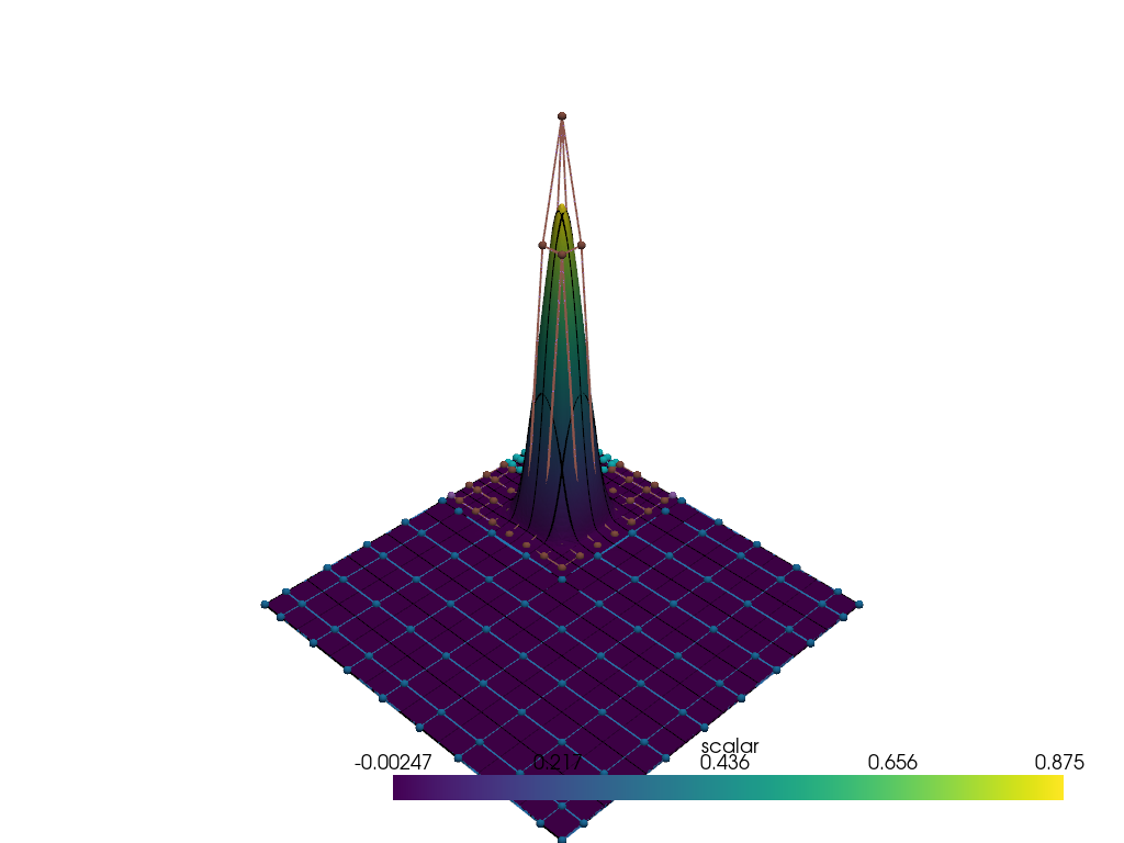
Render the field, hierarchical mesh, and per-level control net

elevation=True lifts the scalar field into a surface; the knot lines are the active-cell boundaries (denser in the refined corner); the control net is drawn per level, coloured by level.

viz.plot(field, elevation=True, show_knot_lines=True, show_control_polygon=True)

Static Scene

Interactive Scene

<pyvista.plotting.plotter.Plotter object at 0x7464c53460f0>

Adaptive refinement loop

Rather than refine a fixed block, let the approximation error drive refinement. Each pass estimates a per-cell error (the peak vs. the current field at cell midpoints), marks the worst cells, refines the space there with refine() (graded and immutable, so it returns a new space), and re-quasi-interpolates. The mesh concentrates on the peak on its own.

adaptive = create_thb_space(root)
approx = quasi_interpolate_thb_spline(peak, adaptive)
for it in range(4):
    cell_lo, cell_hi = adaptive.grid.collect_cell_bounds()
    midpoints = 0.5 * (cell_lo + cell_hi)
    cell_error = np.abs(peak(midpoints) - np.asarray(approx.evaluate(midpoints)))
    marked = np.flatnonzero(cell_error > 0.05 * cell_error.max())
    if marked.size == 0:
        break
    adaptive = adaptive.refine(marked)  # mark -> refine -> new space
    approx = quasi_interpolate_thb_spline(peak, adaptive)
    print(f"pass {it}: {adaptive.num_total_basis} dofs, max cell error {cell_error.max():.2e}")

pass 0: 104 dofs, max cell error 1.35e-01
pass 1: 168 dofs, max cell error 1.97e-02
pass 2: 332 dofs, max cell error 1.87e-02
pass 3: 663 dofs, max cell error 3.65e-03

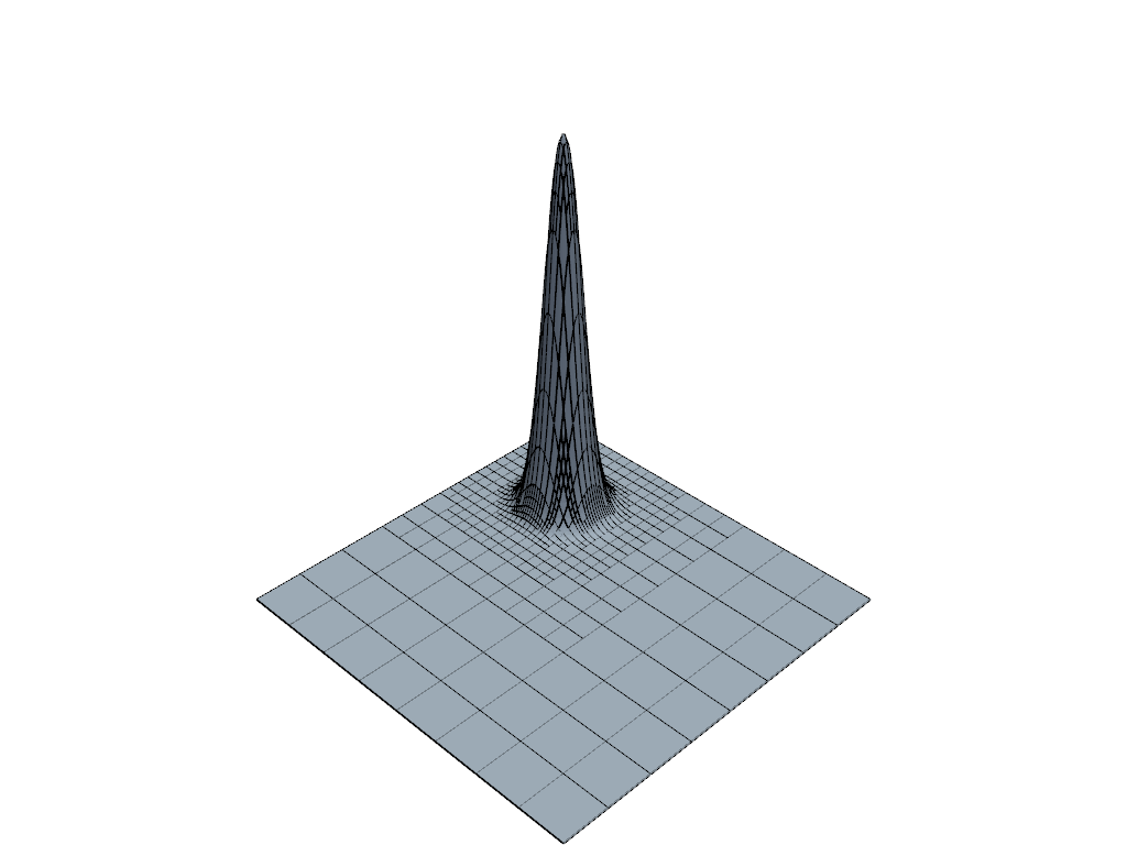
The adapted mesh

The active cells alone make the error-driven refinement structure obvious – fine cells track the peak without the rest of the domain paying for it.

viz.plot(approx, elevation=True, show_knot_lines=True, color="lightsteelblue")

Static Scene

Interactive Scene

<pyvista.plotting.plotter.Plotter object at 0x7464c5344fe0>

Refining a function is exact

refine() / refine_region refine the function (space and coefficients): they return the same field on a finer space. Hierarchical spaces are nested, so the prolongation is exact – this is the lossless field transfer used to carry a solution to a finer mesh inside an adaptive solver.

finer = field.refine_region(0, [0, 0], [8, 8])  # refine the remaining coarse cells
sample = np.random.default_rng(0).random((200, 2))
max_diff = np.abs(finer.evaluate(sample) - field.evaluate(sample)).max()
assert np.allclose(finer.evaluate(sample), field.evaluate(sample))
print(
    f"prolonged {field.space.num_total_basis} -> {finer.space.num_total_basis} dofs; "
    f"field unchanged (max diff {max_diff:.2e})"
)

prolonged 196 -> 372 dofs; field unchanged (max diff 1.51e-15)