Bézier geometry and Bernstein root finding

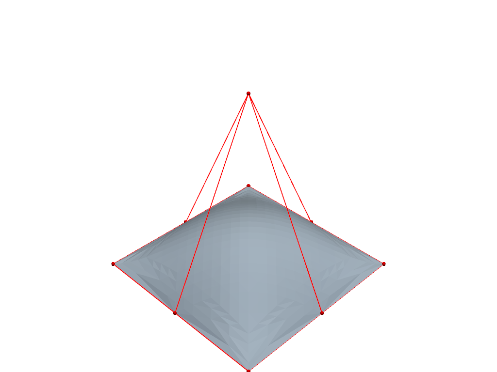
A Bezier stores a single polynomial patch in Bernstein form (its degree comes from the control-point shape) – exactly the per-element pieces produced by to_beziers in Knot operations and Bézier extraction. On top of that representation, find_roots() robustly finds all roots of a scalar 1-D Bézier in [0, 1], selecting its algorithm automatically (Bézier clipping at high degree, an exact derivative-based solver at low degree). This tutorial renders a Bézier surface, locates roots, then uses root finding for a curve-line intersection.

import matplotlib.pyplot as plt
import numpy as np

from pantr import viz
from pantr.bezier import Bezier, find_roots

A Bézier surface

A biquadratic patch defined by its 3x3 control net.

cp = np.zeros((3, 3, 3))
for i in range(3):
    for j in range(3):
        cp[i, j] = [0.5 * i, 0.5 * j, np.sin(np.pi * i / 2) * np.sin(np.pi * j / 2)]
surface = Bezier(cp)
viz.plot(surface, color="lightsteelblue", show_control_polygon=True)

Static Scene

Interactive Scene

<pyvista.plotting.plotter.Plotter object at 0x7464a1deac00>

Roots of a Bernstein polynomial

Build a scalar (rank-1) Bézier whose graph wiggles across zero, then locate every root in [0, 1]. find_roots returns them sorted.

poly = Bezier(np.array([1.0, -3.0, 2.5, -2.0, 1.5])[:, np.newaxis])  # degree-4 scalar
roots = find_roots(poly)

t = np.linspace(0.0, 1.0, 300)
vals = np.asarray(poly.evaluate(t)).reshape(-1)
fig, ax = plt.subplots(figsize=(7, 4), constrained_layout=True)
ax.axhline(0.0, color="0.7")
ax.plot(t, vals, color="navy", lw=2, label="Bernstein polynomial")
ax.plot(roots, np.zeros_like(roots), "o", color="crimson", ms=9, label="roots")
ax.legend()
ax.set_xlabel("t")
ax.set_title(f"find_roots located {len(roots)} roots in [0, 1]")
plt.show()
print("roots:", np.round(roots, 6))

roots: [0.085746 0.72848 ]

Curve–line intersection via roots

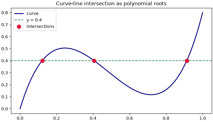
Intersecting a Bézier curve C(t) with the line y = y0 reduces to finding the roots of the scalar polynomial C_y(t) - y0 – itself a Bézier.

curve = Bezier(np.array([[0.0, 0.0], [0.3, 1.5], [0.7, -1.0], [1.0, 0.8]]))
y0 = 0.4
cp_y = curve.control_points[:, 1] - y0
hits_t = find_roots(Bezier(cp_y[:, np.newaxis]))
hits = np.asarray(curve.evaluate(hits_t))

cvals = np.asarray(curve.evaluate(t))
fig, ax = plt.subplots(figsize=(7, 4), constrained_layout=True)
ax.plot(cvals[:, 0], cvals[:, 1], color="navy", lw=2, label="curve")
ax.axhline(y0, color="seagreen", ls="--", label=f"y = {y0}")
ax.plot(hits[:, 0], hits[:, 1], "o", color="crimson", ms=9, label="intersections")
ax.legend()
ax.set_title("Curve-line intersection as polynomial roots")
plt.show()