Your first B-spline

Start here. This tutorial introduces the one idea the rest of PaNTr is built on: a geometry is a function space plus control points.

• a BsplineSpace1D is one knot vector and a degree (a 1-D spline space);

• a BsplineSpace is a tensor product of those 1-D spaces – it fixes the basis and the parametric dimension dim (1 = curve, 2 = surface, 3 = volume);

• a Bspline pairs that space with a control-point array of shape (*num_basis, rank) to give an actual curve/surface/volume. rank is the embedding dimension (2 for a planar curve, 3 in space, 1 for a scalar field).

We build a quadratic curve, evaluate it and its derivative, mark the Greville abscissae, then reuse the same recipe for a surface and for an exact circle (a NURBS). See Core concepts for the full data model and Spaces, knots & element extraction for knot vectors and continuity.

import matplotlib.pyplot as plt
import numpy as np

from pantr import viz
from pantr.bspline import (
    Bspline,
    BsplineSpace,
    BsplineSpace1D,
    create_uniform_space,
    get_greville_abscissae,
)
from pantr.cad import create_circle

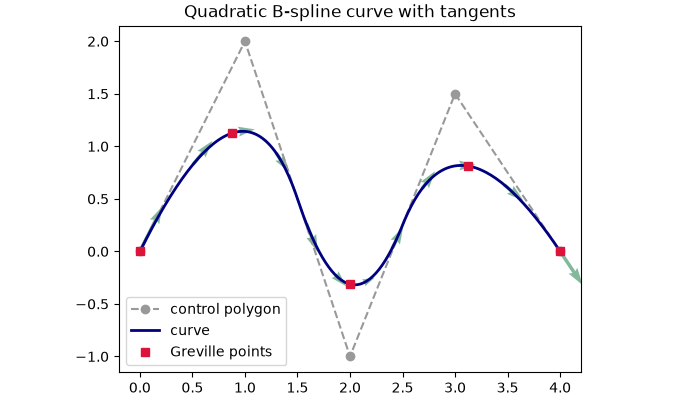
A curve, its control polygon, Greville points, and tangents

The knot vector [0,0,0,1,2,3,3,3] with degree 2 defines a quadratic 1-D space; wrapping it in a (1-direction) BsplineSpace and adding five 2-D control points gives a planar curve (dim == 1, rank == 2). The curve passes near – not through – its control points; the Greville abscissae are the natural parameter values “attached” to each control point. The first derivative is itself a B-spline, evaluated here to draw tangent vectors.

space1d = BsplineSpace1D([0, 0, 0, 1, 2, 3, 3, 3], 2)
control_points = np.array([[0.0, 0.0], [1.0, 2.0], [2.0, -1.0], [3.0, 1.5], [4.0, 0.0]])
curve = Bspline(BsplineSpace([space1d]), control_points)

u = np.linspace(0.0, 3.0, 200)
pts = curve.evaluate(u)
tangents = np.asarray(curve.derivative(0).evaluate(u))
greville = get_greville_abscissae(space1d)
gpts = curve.evaluate(np.asarray(greville, dtype=np.float64))

fig, ax = plt.subplots(figsize=(7, 4), constrained_layout=True)
ax.plot(control_points[:, 0], control_points[:, 1], "o--", color="0.6", label="control polygon")
ax.plot(pts[:, 0], pts[:, 1], color="navy", lw=2, label="curve")
ax.plot(gpts[:, 0], gpts[:, 1], "s", color="crimson", label="Greville points")
qi = np.linspace(0, len(u) - 1, 12).astype(int)
ax.quiver(pts[qi, 0], pts[qi, 1], tangents[qi, 0], tangents[qi, 1], color="seagreen", alpha=0.6)
ax.legend()
ax.set_aspect("equal")
ax.set_title("Quadratic B-spline curve with tangents")
plt.show()

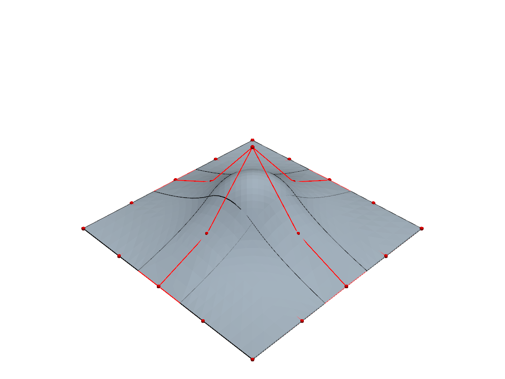
A surface rendered with knot lines and control net

A biquadratic surface over a 3x3 element grid; the control points are lifted by a Gaussian bump. Knot lines show the element boundaries on the surface.

space = create_uniform_space([2, 2], [3, 3])
nu, nv = space.num_basis
gu, gv = np.meshgrid(np.linspace(0, 1, nu), np.linspace(0, 1, nv), indexing="ij")
bump = np.exp(-(((gu - 0.5) ** 2 + (gv - 0.5) ** 2) / 0.05))
surface_cp = np.stack([gu, gv, 0.4 * bump], axis=-1)
surface = Bspline(space, surface_cp)
viz.plot(surface, color="lightsteelblue", show_knot_lines=True, show_control_polygon=True)

Static Scene

Interactive Scene

<pyvista.plotting.plotter.Plotter object at 0x74649bfcd1f0>

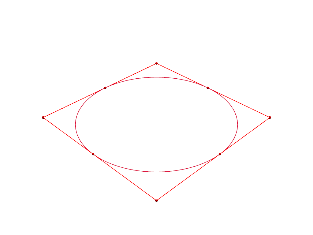
An exact circle (NURBS)

A circle is not a polynomial, but it is a rational quadratic. The control points alternate between the circle and the corners of the circumscribed square; the curve is exact to round-off.

circle = create_circle(radius=1.0)
print("circle is rational:", circle.is_rational)
viz.plot(circle, color="crimson", show_control_polygon=True)

Static Scene

Interactive Scene

circle is rational: True

<pyvista.plotting.plotter.Plotter object at 0x74647fbc0860>