Visualizing geometries

Now that you can build a geometry (Your first B-spline), this tutorial shows how to see it. PaNTr’s pantr.viz module turns B-spline, Bézier, and THB-spline geometries into PyVista meshes backed by native VTK Bézier cells that store the exact polynomial geometry. The interactive viewer below subdivides those cells for display, and a .vtu opened in ParaView (>= 5.10) renders them as exact Bézier cells, tessellated at ParaView’s chosen Nonlinear Subdivision Level. The toolkit is reused throughout the rest of the tutorials:

• plot() – one-call interactive viewing,

• Scene – compose several geometries with per-geometry options,

• control polygons and knot lines overlaid on the geometry,

• scalar fields drawn as a colour map or an elevation surface,

• save() – export to a .vtu file for ParaView.

Requires the viz extra: pip install "pantr[viz]". The Visualization guide covers every rendering option in depth.

import tempfile
from pathlib import Path

import numpy as np

from pantr import viz
from pantr.bspline import Bspline, BsplineSpace, BsplineSpace1D, get_greville_abscissae
from pantr.cad import create_circle, create_disk

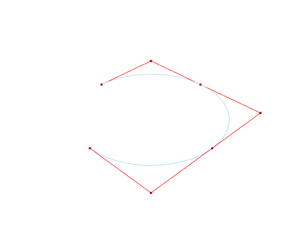
A curve with its control polygon and knot lines

create_circle() builds an exact circle as a rational quadratic (NURBS) curve. show_control_polygon draws the control net; show_knot_lines marks the images of the interior knots.

arc = create_circle(radius=1.0, angle=(0.0, 1.5 * np.pi))
viz.plot(arc, show_control_polygon=True, show_knot_lines=True)

Static Scene

Interactive Scene

<pyvista.plotting.plotter.Plotter object at 0x74649baa1e20>

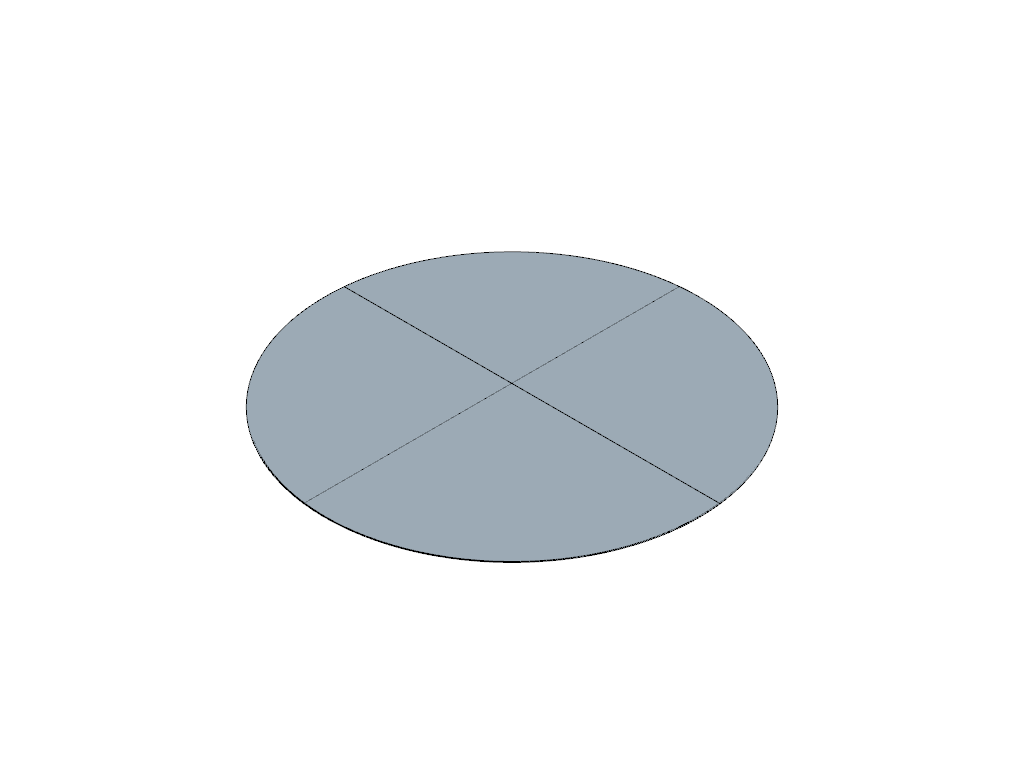
A surface, knot lines on the geometry

For a surface the knot lines become iso-parametric curves lying on the surface.

disk = create_disk(radius_outer=1.0)
viz.plot(disk, color="lightsteelblue", show_knot_lines=True)

Static Scene

Interactive Scene

<pyvista.plotting.plotter.Plotter object at 0x74649baa3f50>

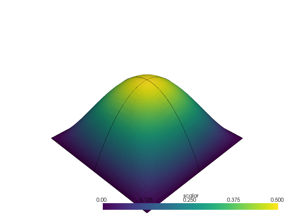
Scalar fields: colour map vs. elevation

A rank-1 geometry is a scalar field f(u, v). By default it is drawn as a flat colour map; elevation=True lifts the value into the third coordinate. Here we build a biquadratic field whose coefficients sample sin(pi u) sin(pi v).

space = BsplineSpace([BsplineSpace1D([0, 0, 0, 0.5, 1, 1, 1], 2) for _ in range(2)])
greville = get_greville_abscissae(space.spaces[0])
gu, gv = np.meshgrid(greville, greville, indexing="ij")
coeffs = (np.sin(np.pi * gu) * np.sin(np.pi * gv))[..., np.newaxis]
field = Bspline(space, coeffs)
viz.plot(field, elevation=True, show_knot_lines=True)

Static Scene

Interactive Scene

<pyvista.plotting.plotter.Plotter object at 0x7464a9fa0560>

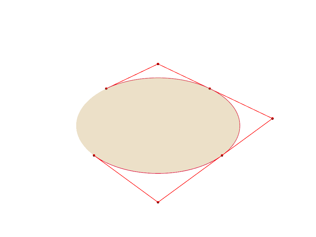
Composing a scene

Scene overlays several geometries, each with its own options.

scene = viz.Scene()
scene.add(disk, color="wheat", opacity=0.5)
scene.add(arc, color="crimson", show_control_polygon=True)
scene.show()

Static Scene

Interactive Scene

<pyvista.plotting.plotter.Plotter object at 0x74649b90a1b0>

Exporting to VTK

save() writes a .vtu file that ParaView (>= 5.10) renders with exact Bézier geometry – handy for publication figures. In ParaView, switch the representation to Surface With Edges to see the knot lines: it draws the cells’ curved edges, dynamically tessellated at the chosen Nonlinear Subdivision Level.

out_file = Path(tempfile.gettempdir()) / "pantr_disk.vtu"
viz.save(disk, out_file)
print(f"wrote {out_file}")

wrote /tmp/pantr_disk.vtu