Polynomial bases and change of basis

Every spline is a linear combination of basis functions. pantr.basis tabulates the common 1-D polynomial bases used to build spline and finite-element spaces, and pantr.change_basis provides the exact matrices that convert coefficients between them. This tutorial plots the bases at a fixed degree and visualizes one such change-of-basis matrix.

Each tabulate_*_1d call returns an (n_points, degree + 1) array whose columns are the individual basis functions sampled at the supplied points. The same bases appear element-locally in SpanwiseElementExtraction (Spaces, knots & element extraction).

import matplotlib.pyplot as plt
import numpy as np

from pantr.basis import (
    LagrangeVariant,
    tabulate_bernstein_1d,
    tabulate_lagrange_1d,
    tabulate_legendre_1d,
)
from pantr.change_basis import compute_bernstein_to_lagrange_1d

DEGREE = 4
x = np.linspace(0.0, 1.0, 200)

Four bases at degree 4

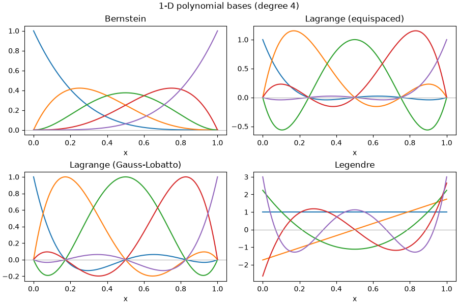
Bernstein (non-negative, partition of unity), Lagrange on equispaced nodes (interpolatory – each function is 1 at its node, 0 at the others), Lagrange on Gauss-Lobatto-Legendre nodes (clustered at the ends, much better conditioned), and the Legendre polynomials (orthogonal on [0, 1]).

bases = {
    "Bernstein": tabulate_bernstein_1d(DEGREE, x),
    "Lagrange (equispaced)": tabulate_lagrange_1d(DEGREE, LagrangeVariant.EQUISPACES, x),
    "Lagrange (Gauss-Lobatto)": tabulate_lagrange_1d(
        DEGREE, LagrangeVariant.GAUSS_LOBATTO_LEGENDRE, x
    ),
    "Legendre": tabulate_legendre_1d(DEGREE, x),
}

fig, axes = plt.subplots(2, 2, figsize=(9, 6), constrained_layout=True)
for ax, (name, table) in zip(axes.ravel(), bases.items(), strict=True):
    ax.plot(x, table)
    ax.set_title(name)
    ax.axhline(0.0, color="0.7", lw=0.8)
    ax.set_xlabel("x")
fig.suptitle(f"1-D polynomial bases (degree {DEGREE})")
plt.show()

Change of basis

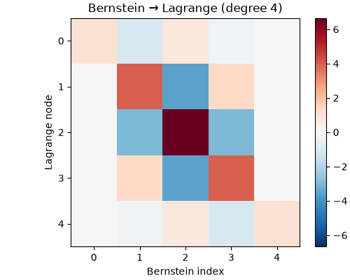
pantr.change_basis builds the matrices that convert coefficients between bases. compute_bernstein_to_lagrange_1d maps Bernstein coefficients to Lagrange (nodal) values: row i is the Bernstein basis evaluated at node i.

matrix = np.asarray(compute_bernstein_to_lagrange_1d(DEGREE, LagrangeVariant.EQUISPACES))

fig, ax = plt.subplots(figsize=(5, 4), constrained_layout=True)
im = ax.imshow(matrix, cmap="RdBu_r", vmin=-abs(matrix).max(), vmax=abs(matrix).max())
ax.set_title(f"Bernstein → Lagrange (degree {DEGREE})")
ax.set_xlabel("Bernstein index")
ax.set_ylabel("Lagrange node")
fig.colorbar(im, ax=ax)
plt.show()

Partition of unity

The Bernstein basis is non-negative and sums to one at every point – the property behind the convex-hull bound of a control polygon. (Lagrange bases also sum to one but may be negative; Legendre polynomials do not sum to one.)

print("max |sum of Bernstein - 1| =", float(np.abs(bases["Bernstein"].sum(axis=1) - 1.0).max()))

max |sum of Bernstein - 1| = 5.551115123125783e-16