Approximation: interpolation, fitting, projection, quasi-interpolation

So far the control points have come from geometry we built directly – placed by hand or produced by the CAD module. Often the geometry is the unknown instead: given a function (or sampled data), find the spline that best represents it. pantr.bspline offers several routes, trading cost against accuracy: interpolate_bspline() (match the function at the Greville points by default), l2_project_bspline() (best \(L^2\) fit), and quasi_interpolate_bspline() (a cheap, purely local projector). This tutorial compares them on a fixed space and shows \(L^2\) convergence under refinement.

Note the calling conventions: interpolate_bspline and l2_project_bspline call func(lattice) (a PointsLattice, use lattice.pts_per_dir), while quasi_interpolate_bspline calls func(points) with a flat (M, dim) array.

import matplotlib.pyplot as plt
import numpy as np

from pantr.bspline import (
    create_uniform_space,
    interpolate_bspline,
    l2_project_bspline,
    quasi_interpolate_bspline,
)


def g(x):
    """The 1-D target function on [0, 1]."""
    return np.exp(np.sin(3.0 * np.pi * np.asarray(x)))


# Adapters for the two calling conventions (1-D, so just the first axis).
def on_lattice(lattice):
    return g(lattice.pts_per_dir[0])


def on_points(points):
    return g(points[:, 0])

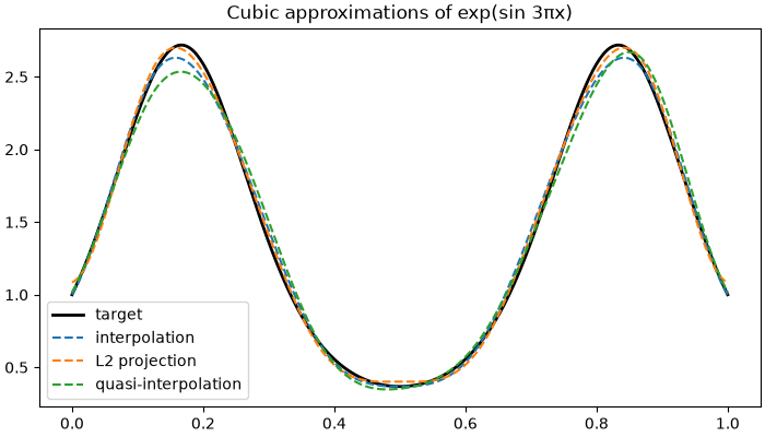
Three approximations on the same space

space = create_uniform_space([3], [8])  # cubic, 8 elements
approx = {
    "interpolation": interpolate_bspline(on_lattice, space),
    "L2 projection": l2_project_bspline(on_lattice, space),
    "quasi-interpolation": quasi_interpolate_bspline(on_points, space),
}

x = np.linspace(0.0, 1.0, 400)
fx = g(x)
fig, ax = plt.subplots(figsize=(7, 4), constrained_layout=True)
ax.plot(x, fx, "k", lw=2, label="target")
for name, spline in approx.items():
    ax.plot(x, np.asarray(spline.evaluate(x)).reshape(-1), "--", label=name)
ax.legend()
ax.set_title("Cubic approximations of exp(sin 3πx)")
plt.show()

L2 convergence under refinement

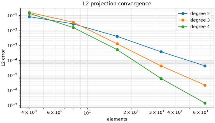
Refining the mesh drives the L2 projection error down at the optimal rate for the degree. We estimate the error by dense sampling.

def l2_error(spline):
    vals = np.asarray(spline.evaluate(x)).reshape(-1)
    return float(np.sqrt(np.trapezoid((vals - fx) ** 2, x)))


n_elements = [4, 8, 16, 32, 64]
fig, ax = plt.subplots(figsize=(7, 4), constrained_layout=True)
for p in (2, 3, 4):
    errors = [
        l2_error(l2_project_bspline(on_lattice, create_uniform_space([p], [n]))) for n in n_elements
    ]
    ax.loglog(n_elements, errors, "o-", label=f"degree {p}")
ax.set_xlabel("elements")
ax.set_ylabel("L2 error")
ax.legend()
ax.grid(True, which="both", alpha=0.3)
ax.set_title("L2 projection convergence")
plt.show()

degree4_errors = errors  # last loop iteration (p=4); captured for testing